Introduction
This script trains an agent with stochastic policy gradient ascent to solve the Lunar Lander challenge from OpenAI.
In order to run this script, NumPy, the OpenAI Gym toolkit, and PyTorch will need to be installed.
Each step through the Lunar Lander environment takes the general form:
state, reward, done, info = env.step(action)
and the goal is for the agent to take actions that maximize the cumulative reward achieved for the episode's duration. In this specific environment, the state space is 8-dimensional and continuous, while the action space consists of four discrete options:
- do nothing,
- fire the left orientation engine,
- fire the main engine,
- and fire the right orientation engine.
In order to "solve" the environment, the agent needs to complete the episode with at least 200 points. To learn more about how the agent receives rewards, see here.
Algorithm
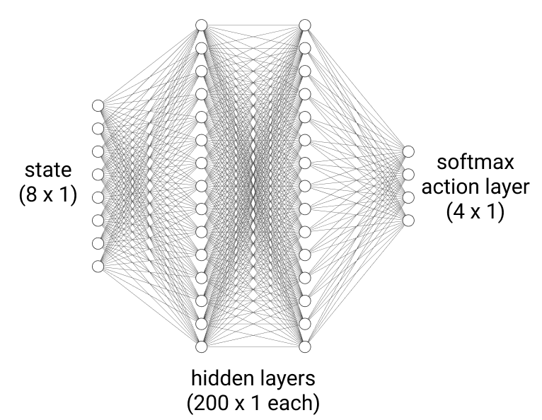
Since the agent can only take one of four actions, a, at each time step t, a natural choice of policy would yield probabilities of each action as its output, given an input state, s. Namely, the policy, πθ(a|s), chosen for the agent is a neural network function approximator, designed to more closely approximate the optimal policy π*(a|s) of the agent as it trains over more and more episodes. Here, θ represents the parameters of the neural network that are initially randomized but improve over time to produce more optimal actions, meaning those actions that lead to more cumulative reward over time. Each hidden layer of the neural network uses a ReLU activation. The last layer is a softmax layer of four neurons, meaning each neuron outputs the probability that its corresponding action will be selected.
Now that the agent has a stochastic mechanism to select output actions given an input state, it begs the question as to how the policy itself improves over episodes. At the end of each episode, the reward, Gt, due to selecting a specific action, at, at time t during the episode can be expressed as follows:
Gt = rt + (γ)rt+1 + (γ2)rt+2 + ...
where rt is the immediate reward and all remaining terms form the discounted sum of future rewards with discount factor 0 < γ < 1.
Then, the goal is to change the parameters to increase the expectation of future rewards. By taking advantage of likelihood ratios, a gradient estimator of the form below can be used:
grad = Et [ ∇θ log( πθ( at | st ) ) Gt ]
where the advantage function is given by the total reward Gt produced by the action at. Updating the parameters in the direction of the gradient has the net effect of increasing the likelihood of taking actions that were eventually rewarded and decreasing the likelihood of taking actions that were eventually penalized. This is possible because Gt takes into account all the future rewards received as well as the immediate reward.
Results
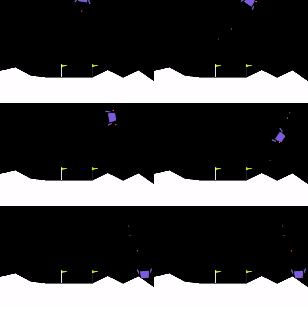
Solving the Lunar Lander challenge requires safely landing the spacecraft between two flag posts while consuming limited fuel. The agent's ability to do this was quite abysmal in the beginning.
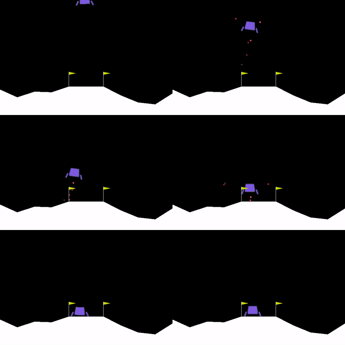
After training the agent overnight on a GPU, it could gracefully complete the challenge with ease!
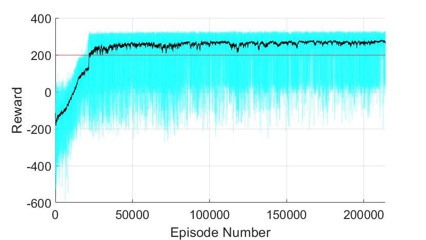
Below, the performance of the agent over 214,000 episodes is documented. The light-blue line indicates individual episodic performance, and the black line is a 100-period moving average of performance. The red line marks the 200 point success threshold.
It took a little over 17,000 episodes before the agent completed the challenge with a total reward of at least 200 points. After around 25,000 episodes, its average performance began to stabilize, yet, it should be noted that there remained a high amount of variance between individual episodes. In particular, even within the last 15,000 episodes of training, the agent failed roughly 5% of the time. Although the agent could easily conquer the challenge, it occasionally could not prevent making decisions that would eventually lead to disastrous consequences.
Discussion
One caveat with this specific implementation is that it only works with a discrete action space. However, it is possible to adapt the same algorithm to work with a continuous action space. In order to do so, the softmax output layer would have to transform into a sigmoid or tanh layer, nulling the idea that the output layer corresponds to probabilities. Each output neuron would now correspond to the mean, μ, of the (assumed) Gaussian distribution to which each action belongs. In essence, the distributional means themselves would be functions of the input state.
The training process would then consist of updating parameters such that the means shift to favor actions that result in eventual rewards and disfavor actions that are eventually penalized. While it is possible to adapt the algorithm to support continuous action spaces, it has been noted to have relatively poor or limited performance in practice. In actual scenarios involving continuous action spaces, it would almost certainly be preferable to use DDPG, PPO, or a similar algorithm.
References
- Introduction to Reinforcement Learning - David Silver
- Deep Reinforcement Learning: Pong from Pixels - Andrej Karpathy
- The Likelihood-Ratio Gradient - Tim Vieira
- Policy Gradient Loss with Continuous Action Spaces - Stack Overflow Post
- Continuous Control With Deep Reinforcement Learning - Timothy P. Lillicrap et al.
- Proximal Policy Optimization Algorithms - John Schulman et al.
License
All files in the repository are under the MIT license.
