Differentiable Optimizers with Perturbations in PyTorch
This contains a PyTorch implementation of Differentiable Optimizers with Perturbations in Tensorflow. All credit belongs to the original authors which can be found below. The source code, tests, and examples given below are a one-to-one copy of the original work, but with pure PyTorch implementations.
Overview
We propose in this work a universal method to transform any optimizer in a differentiable approximation. We provide a PyTorch implementation, illustrated here on some examples.
Perturbed argmax
We start from an original optimizer, an argmax function, computed on an example input theta.
import torch
import torch.nn.functional as F
import perturbations

device = torch.device("cuda:0" if torch.cuda.is_available() else "cpu")

def argmax(x, axis=-1):
    return F.one_hot(torch.argmax(x, dim=axis), list(x.shape)[axis]).float()
This function returns a one-hot corresponding to the largest input entry.
>>> argmax(torch.tensor([-0.6, 1.9, -0.2, 1.1, -1.0]))
tensor([0., 1., 0., 0., 0.])
It is possible to modify the function by creating a perturbed optimizer, using Gumbel noise.
pert_argmax = perturbations.perturbed(argmax,
                                      num_samples=1000000,
                                      sigma=0.5,
                                      noise='gumbel',
                                      batched=False,
                                      device=device)
>>> theta = torch.tensor([-0.6, 1.9, -0.2, 1.1, -1.0], device=device)
>>> pert_argmax(theta)
tensor([0.0055, 0.8150, 0.0122, 0.1648, 0.0025], device='cuda:0')
In this particular case, it is equal to the usual softmax with exponential weights.
>>> sigma = 0.5
>>> F.softmax(theta/sigma, dim=-1)
tensor([0.0055, 0.8152, 0.0122, 0.1646, 0.0025], device='cuda:0')
Batched version
The original function can accept a batch dimension, and is applied to every element of the batch.
theta_batch = torch.tensor([[-0.6, 1.9, -0.2, 1.1, -1.0],
                            [-0.6, 1.0, -0.2, 1.8, -1.0]], device=device, requires_grad=True)
>>> argmax(theta_batch)
tensor([[0., 1., 0., 0., 0.],
        [0., 0., 0., 1., 0.]], device='cuda:0')
Likewise, if the argument batched is set to True (its default value), the perturbed optimizer can handle a batch of inputs.
pert_argmax = perturbations.perturbed(argmax,
                                      num_samples=1000000,
                                      sigma=0.5,
                                      noise='gumbel',
                                      batched=True,
                                      device=device)
>>> pert_argmax(theta_batch)
tensor([[0.0055, 0.8158, 0.0122, 0.1640, 0.0025],
        [0.0066, 0.1637, 0.0147, 0.8121, 0.0030]], device='cuda:0')
It can be compared to its deterministic version, the softmax.
>>> F.softmax(theta_batch/sigma, dim=-1)
tensor([[0.0055, 0.8152, 0.0122, 0.1646, 0.0025],
        [0.0067, 0.1639, 0.0149, 0.8116, 0.0030]], device='cuda:0')
Decorator version
It is also possible to use the perturbed function as a decorator.
@perturbations.perturbed(num_samples=1000000, sigma=0.5, noise='gumbel', batched=True, device=device)
def argmax(x, axis=-1):
  	return F.one_hot(torch.argmax(x, dim=axis), list(x.shape)[axis]).float()
>>> argmax(theta_batch)
tensor([[0.0054, 0.8148, 0.0121, 0.1652, 0.0024],
        [0.0067, 0.1639, 0.0148, 0.8116, 0.0029]], device='cuda:0')
Gradient computation
The Perturbed optimizers are differentiable, and the gradients can be computed with stochastic estimation automatically. In this case, it can be compared directly to the gradient of softmax.
output = pert_argmax(theta_batch)
square_norm = torch.linalg.norm(output)
square_norm.backward(torch.ones_like(square_norm))
grad_pert = theta_batch.grad
>>> grad_pert
tensor([[-0.0072,  0.1708, -0.0132, -0.1476, -0.0033],
        [-0.0068, -0.1464, -0.0173,  0.1748, -0.0046]], device='cuda:0')
Compared to the same computations with a softmax.
output = F.softmax(theta_batch/sigma, dim=-1)
square_norm = torch.linalg.norm(output)
square_norm.backward(torch.ones_like(square_norm))
grad_soft = theta_batch.grad
>>> grad_soft
tensor([[-0.0064,  0.1714, -0.0142, -0.1479, -0.0029],
        [-0.0077, -0.1457, -0.0170,  0.1739, -0.0035]], device='cuda:0')
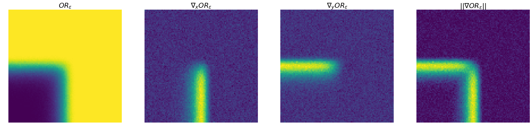
Perturbed OR
The OR function over the signs of inputs, that is an example of optimizer, offers a well-interpretable visualization.
def hard_or(x):
    s = ((torch.sign(x) + 1) / 2.0).type(torch.bool)
    result = torch.any(s, dim=-1)
    return result.type(torch.float) * 2.0 - 1
In the following batch of two inputs, both instances are evaluated as True (value 1).
theta = torch.tensor([[-5., 0.2],
                      [-5., 0.1]], device=device)
>>> hard_or(theta)
tensor([1., 1.])
Computing a perturbed OR operator over 1000 samples shows the difference in value for these two inputs.
pert_or = perturbations.perturbed(hard_or,
                                  num_samples=1000,
                                  sigma=0.1,
                                  noise='gumbel',
                                  batched=True,
                                  device=device)
>>> pert_or(theta)
tensor([1.0000, 0.8540], device='cuda:0')
This can be vizualized more broadly, for values between -1 and 1, as well as the evaluated values of the gradient.
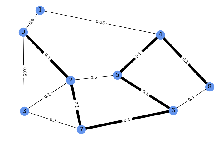
Perturbed shortest path
This framework can also be easily applied to more complex optimizers, such as a blackbox shortest paths solver (here the function shortest_path). We consider a small example on 9 nodes, illustrated here with the shortest path between 0 and 8 in bold, and edge costs labels.
We also consider a function of the perturbed solution: the weight of this solution on the edgebetween nodes 6 and 8.
A gradient of this function with respect to a vector of four edge costs (top-rightmost, between nodes 4, 5, 6, and 8) is automatically computed. This can be used to increase the weight on this edge of the solution by changing these four costs. This is challenging to do with first-order methods using only an original optimizer, as its gradient would be zero almost everywhere.
final_edges_costs = torch.tensor([0.4, 0.1, 0.1, 0.1], device=device, requires_grad=True)
weights = edge_costs_to_weights(final_edges_costs)

@perturbations.perturbed(num_samples=100000, sigma=0.05, batched=False, device=device)
def perturbed_shortest_path(weights):
    return shortest_path(weights, symmetric=False)
We obtain a perturbed solution to the shortest path problem on this graph, an average of solutions under perturbations on the weights.
>>> perturbed_shortest_path(weights)
tensor([[0.    0.    0.001 0.025 0.    0.    0.    0.    0.   ]
        [0.    0.    0.    0.    0.023 0.    0.    0.    0.   ]
        [0.679 0.    0.    0.119 0.    0.    0.    0.    0.   ]
        [0.304 0.    0.    0.    0.    0.    0.    0.    0.   ]
        [0.    0.023 0.    0.    0.    0.898 0.    0.    0.   ]
        [0.    0.    0.001 0.    0.    0.    0.896 0.    0.   ]
        [0.    0.    0.    0.    0.    0.001 0.    0.974 0.   ]
        [0.    0.    0.797 0.178 0.    0.    0.    0.    0.   ]
        [0.    0.    0.    0.    0.921 0.    0.079 0.    0.   ]])
For illustration, this solution can be represented with edge width proportional to the weight of the solution.
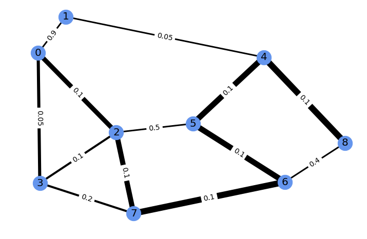
We consider an example of scalar function on this solution, here the weight of the perturbed solution on the edge from node 6 to 8 (of current value 0.079).
def i_to_j_weight_fn(i, j, paths):
    return paths[..., i, j]

weights = edge_costs_to_weights(final_edges_costs)
pert_paths = perturbed_shortest_path(weights)
i_to_j_weight = pert_paths[..., 8, 6]
i_to_j_weight.backward(torch.ones_like(i_to_j_weight))
grad = final_edges_costs.grad
This provides a direction in which to modify the vector of four edge costs, to increase the weight on this solution, obtained thanks to our perturbed version of the optimizer.
>>> grad
tensor([-2.0993764,  2.076386 ,  2.042395 ,  2.0411625], device='cuda:0')
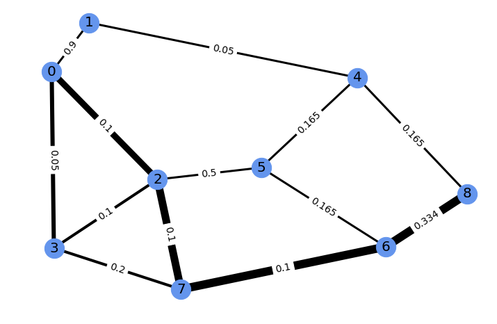
Running gradient ascent for 30 steps on this vector of four edge costs to increase the weight of the edge from 6 to 8 modifies the problem. Its new perturbed solution has a corresponding edge weight of 0.989. The new problem and its perturbed solution can be vizualized as follows.
References
Berthet Q., Blondel M., Teboul O., Cuturi M., Vert J.-P., Bach F., Learning with Differentiable Perturbed Optimizers, NeurIPS 2020
License
Please see the original repository for proper details.
 141 Oct 6, 2022

 269 Nov 15, 2022

 91 Nov 21, 2022
 338 Dec 28, 2022
 3 Oct 15, 2022
 68 Dec 29, 2022
 114 Dec 27, 2022
 44 Dec 10, 2022
 118 Dec 6, 2022

 621 Jan 8, 2023
 302 Dec 14, 2022
 46 Nov 17, 2022
 48 Sep 19, 2022
 6 Jun 24, 2022
 76 Jan 2, 2023
 7.6k Jan 4, 2023
 655 Jan 4, 2023
 170 Dec 27, 2022